A concise tutorial on recommender systems

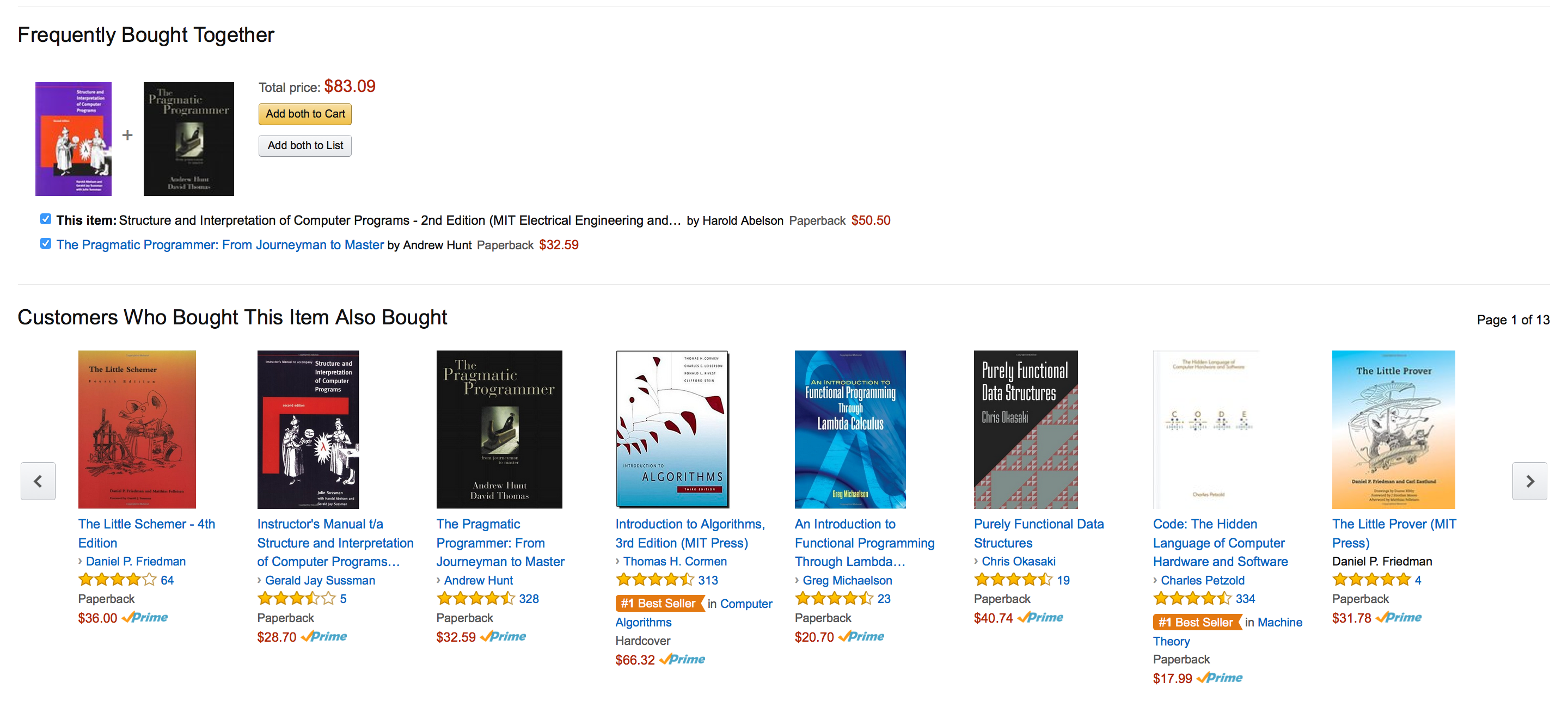
A recommender system predicts the likelihood that a user would prefer an item. Based on previous user interaction with the data source that the systems takes the information from (besides the data from other users, or historical trends), the system is capable to recommend an item to a user. Think about the fact that Amazon recommends you books that they think you could like; Amazon might be making effective use of a recommender system behind the curtains. This simple definition, allows us to think in a diverse set of applications where recommender systems might be useful. Applications such as documents, movies, music, romantic partners, or who to follow on Twitter, are pervasive and widely known in the world of Information Retrieval.

_config.yml

Such amazing applications, carries a huge amount of theory behind them. While theory can be a little bit intimidating and dry, basic understanding of data structures, a programming language, and a little bit of abstraction is all you need to understand the basics of recommender systems.

In this tutorial, We will help you gain a basic understanding on collaborative based Recommender Systems, by building the most basic recommender system out there. We hope that this tutorial motivates you to find out more about Recommender Systems, both in theory and practice. The prerequisites to reading this tutorial are knowledge of a programming language (we’ll use Python, but if you know how does Hash Maps and List works, that’s ok), and a little bit of high-school algebra. You do not need to have prior exposure to recommender systems.

This tutorial makes use of a class of RS (Recommender System) algorithm called collaborative filtering. A collaborative filtering algorithm works by finding a set of people (assuming persons are the only client or user of a RS) with preferences or tastes similar to the target user. Using this smaller set of “similar” people, it constructs a ranked list of suggestions. There’re are several ways to measure the similarity of two people. It’s important to highlight that we’re not going to use attributes or descriptors of an item to recommend it, we’re just using the tastes or preferences over that item.

Assuming that our users are people, and our items are simply that: items, we need to organise our data to ease the processing step. We’re assuming that the data fits in memory, and that you can organise the data as follows.

_config.yml

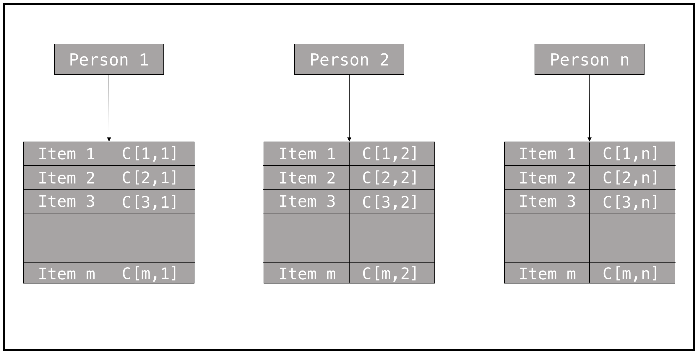
The data structure that we are going to use, consists of people pointing to a dictionary whose keys are the items, and values are the numeric preference of each person on this item. If a person has never ranked the item, C[i, j], is null. In this notation C[i, j] represents the numeric rating of Person j, over the Item i. No matter how the rating is expressed, we need to convert them to numeric values. A sample data structure for our working example is the following definition of a Python dictionary, it includes some ratings of people to computer science related books.

data = {
	'Alan Perlis': { 
		'Artificial intelligence': 1.46, 
		'Systems programming': 5.0, 
		'Software engineering': 3.34, 
		'Databases': 2.32
	},

	'Marvin Minsky': { 
		'Artificial intelligence': 5.0, 
		'Systems programming': 2.54,
		'Computation': 4.32, 
		'Algorithms': 2.76
	},

	'John McCarthy': { 
		'Artificial intelligence': 5.0, 
		'Programming language theory': 4.72, 
		'Systems programming': 3.25, 
		'Concurrency': 3.61, 
		'Formal methods': 3.58,
		'Computation': 3.23, 
		'Algorithms': 3.03 
	},

	'Edsger Dijkstra': { 
		'Programming language theory': 4.34, 
		'Systems programming': 4.52,
		'Software engineering': 4.04, 
		'Concurrency': 3.97,
		'Formal methods': 5.0, 
		'Algorithms': 4.92 
	},

	'Donald Knuth': { 
		'Programming language theory': 4.33, 
		'Systems programming': 3.57,
		'Computation': 4.39, 
		'Algorithms': 5.0 
	},

	'John Backus': { 
		'Programming language theory': 4.58, 
		'Systems programming': 4.43,
		'Software engineering': 4.38, 
		'Formal methods': 2.42, 
		'Databases': 2.80 
	},

	'Robert Floyd': { 
		'Programming language theory': 4.24, 
		'Systems programming': 2.17,
		'Concurrency': 2.92, 
		'Formal methods': 5.0, 
		'Computation': 3.18, 
		'Algorithms': 5.0 
	},

	'Tony Hoare': { 
		'Programming language theory': 4.64, 
		'Systems programming': 4.38,
		'Software engineering': 3.62, 
		'Concurrency': 4.88,
		'Formal methods': 4.72, 
		'Algorithms': 4.38
	},

	'Edgar Codd': { 
		'Systems programming': 4.60, 
		'Software engineering': 3.54,
		'Concurrency': 4.28, 
		'Formal methods': 1.53, 
		'Databases': 5.0
	},

	'Dennis Ritchie': { 
		'Programming language theory': 3.45, 
		'Systems programming': 5.0,
		'Software engineering': 4.83,
	},

	'Niklaus Wirth': { 
		'Programming language theory': 4.23, 
		'Systems programming': 4.22,
		'Software engineering': 4.74, 
		'Formal methods': 3.83, 
		'Algorithms': 3.95
	},

	'Robin Milner': { 
		'Programming language theory': 5.0, 
		'Systems programming': 1.66,
		'Concurrency': 4.62, 
		'Formal methods': 3.94,
	},

	'Leslie Lamport': { 
		'Programming language theory': 1.5, 
		'Systems programming': 2.76,
		'Software engineering': 3.76, 
		'Concurrency': 5.0,
		'Formal methods': 4.93, 
		'Algorithms': 4.63
	},

	'Michael Stonebraker': { 
		'Systems programming': 4.67, 
		'Software engineering': 3.86,
		'Concurrency': 4.14, 
		'Databases': 5.0,
	},
}

In this example, Leslie Lamport, rates the book Software engineering with 3.76, while Robin Milner, rates the Programming language theory book with 5.0. A simple problem that we might want to solve using this dataset and a recommender system, is how likely Marvin Minsky is to like the title Programming language theory. In order to solve this kind of problems, we do need a way to measure how similar people are based on their rankings. A naive but popular approach is to compare every pair and find a similarity score; now the problem is to find an adequate similarity score. The most common approaches to the similarity problem, are score by Euclidean Distance, and using the Pearson Correlation Coefficient; both terms are deeply related to statistics and linear algebra.

Euclidean distance score

The Euclidean distance between two points is the length of the line segments connecting them. Our Euclidean space in this particular case is the positive portion of the plane where the axes are the ranked items and the points represent the scores that a particular person gives to both items. Two people belongs to a certain preference space if and only if, they have ranked the two items that defines the preference space. So we define a preference space for each pair of distinct items, and the points in this preference space, are given by the people that ranked the two items. To visualise this idea, we consider the preference space, defined by the items Systems programming, and Programming language theory.

_config.yml

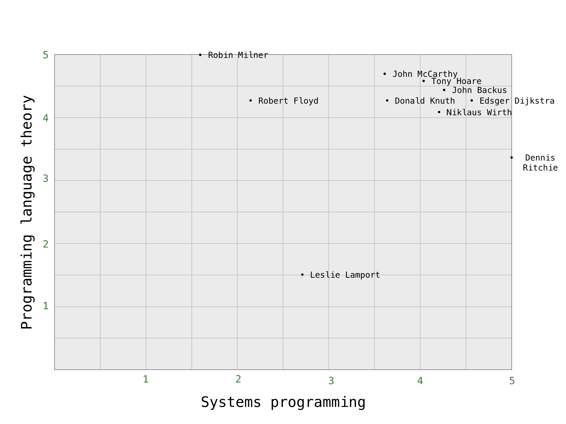
The figure shows the people that have ranked both items in a preference space defined by those items, and the scores given by the people to each item independently. In the chart, Leslie Lamport appears that low since he has ranked Systems programming with 2.76 and Programming language theory with 1.5. We can clearly see that regarding this items, John McCarthy, and Tony Hoare are pretty similar, while Robin Milner and Bob Floyd are slightly different; Dennis Ritchie and Leslie Lamport have little in common (regarding those items). We can now proceed to define the distance between two people in the preference space as we define the distance between a pair of points in the plane:

$d(Person_i,\ Person_j) = \sqrt{(X_1 - X_2)^2 +(Y_1 - Y2)^2}$

If $d(Person_i,\ Person_j)$ is small, then $Person_i$ is similar to $Person_j$ . Since we do want a metric that tell us how similar two people are; that is a bigger number might represent more similarity, we are required to take a normalised value based on $d(Person_i,\ Person_j)$ . Our final similarity metric based on Euclidean distance is:

$\frac{1}{\left[ 1 + d(Person_i,\ Person_j) \right]}\ \in [0,\ 1]$

This formula is designed thinking in division by zero and the proportionality that we need.

The closest to one this metric is, the closest $Person_i$ is to $Person_j$ by similarity. If we extend this idea to the set of ranked items in common for two people, we can design an algorithm that tell us the similarity of a pair based on their tastes. We just need the common items between two people and get this metric for every common distinct pair. The following algorithm, computes the Euclidean Similarity between two people based on their common tastes. Those tastes are retrieved from our main data structure stored in our data variable.

def euclidean_similarity(person1, person2):

    common_ranked_items = [itm for itm in data[person1] \
        if itm in data[person2]]
		
    rankings = [(data[person1][itm], data[person2][itm]) \
        for itm in common_ranked_items]
		
    distance = [pow(rank[0] - rank[1], 2) for rank in rankings]

    return 1 / (1 + sum(distance))

Once we have the data and the algorithm, we can analyse it. The major flaw of this algorithm, and in general of Euclidean distance based comparisons, is that if the whole distribution of rankings from a person tend to be higher than those from other person (a person is inclined to give higher scores than the other), this metric would classify them as disimilar without regard the correlation between two people. There can still be perfect correlation if the differences between their rankings is consistent. While a clever algorithm would classify them as similar, our Euclidean based algorithm, will say that two people are very different because one is consistently harsher then the other one. That behaviour depends on the application of the recommender system (thus far, we have not created a recommender system; we’re just computing similarity).

Pearson correlation coefficient

In statistics, the Pearson correlation coefficient is a measure of the linear dependence or correlation between two variables X and Y. It has a value between +1 and −1 inclusive, where 1 is total positive linear correlation, 0 is no linear correlation, and −1 is total negative linear correlation. In the case of recommender systems, we’re supposed to figure it out how related two people are based on the items they both have ranked. The Pearson correlation coefficient (PCC) is better understood in this case as a measure of the slope of two datasets related by a single line (we’re not taking into account dimensions). The derivation and the formula itself are harder to find and understand, but by using this method, we’re eliminating the weight of harshness while measuring the relation between two people.

The PCC algorithm, requires two datasets as inputs, those datasets don’t come from how people ranked the items, but they come from the common ranked items between two people. PCC help us to find the similarity of a pair of users. Rather than considering the distance between the rankings on two products, we can consider the correlation between the users ratings.

To clarify the concept of correlation, we include a new dataset and some charts. The dataset, includes few ratings of some remarkable computer scientists to some CS books.

_config.yml

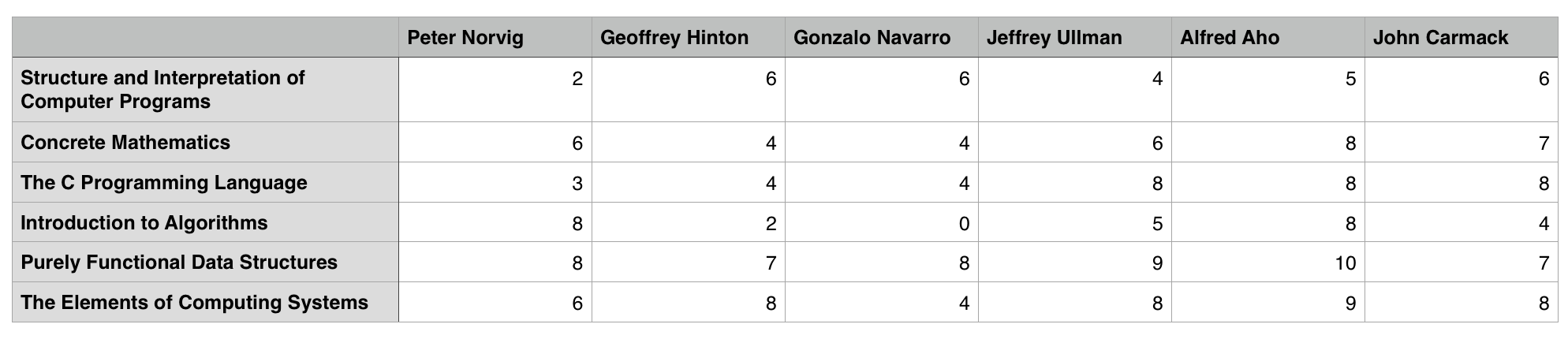
In order to understand how related are two people, we proceed by plotting their preferences (treating each book as a point, whose coordinates are determined by the rating on this item by both users). Once we have that specific plot, we do need to find the best fit straight line over those points. Finding such a line, requires knowledge of linear regression, a topic that’s out of the scope of this tutorial. While finding the best fit straight line, is not as trivial as it seems, finding the PCC depends just on the data that we already have. This best fit line serves us to explain the concept.

_config.yml

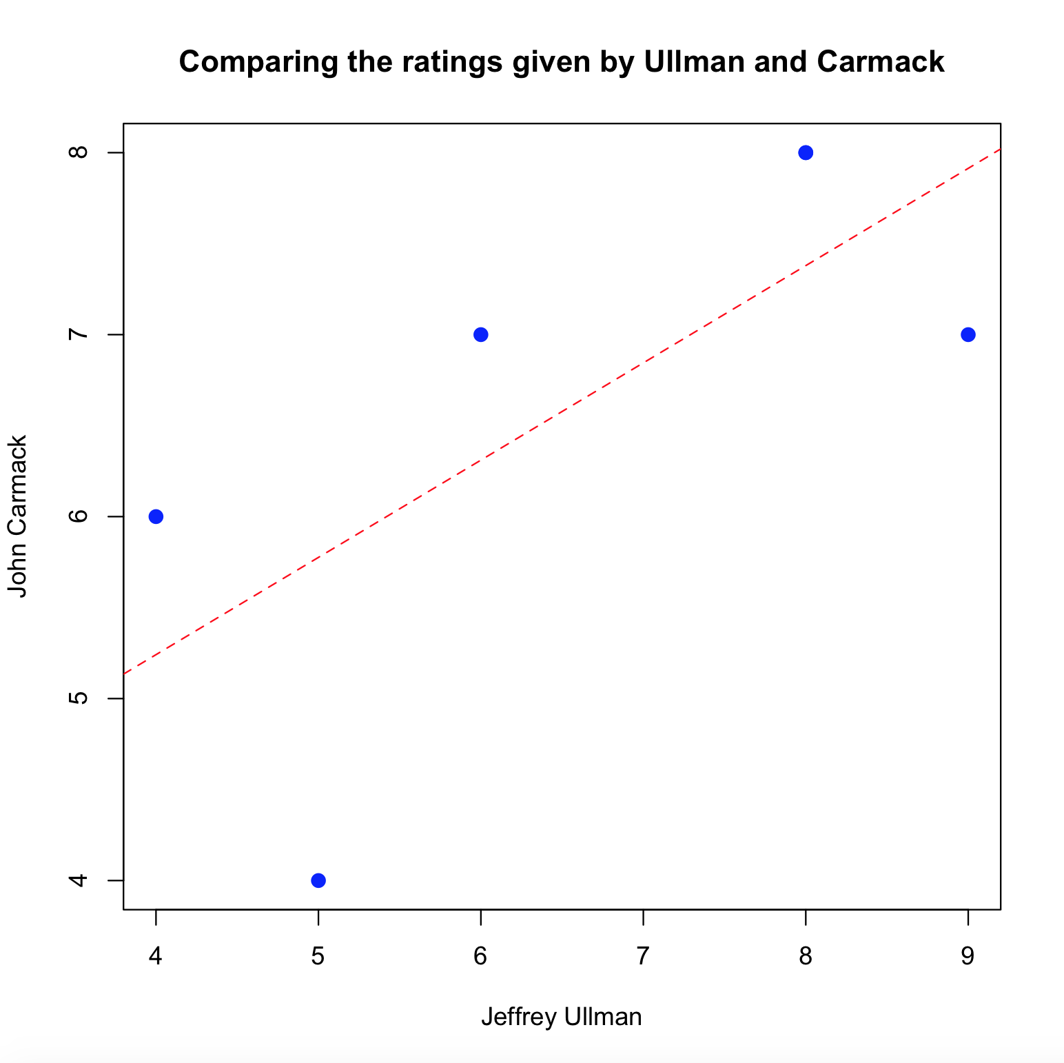
The plot shows the 2-dimensional space defined by the ratings of Ullman and `Carmack, as well as the best fit straight line. The positive slope of the line, shows a positive correlation between those points, then, the PCC for Ullman and Carmack is positive.

_config.yml

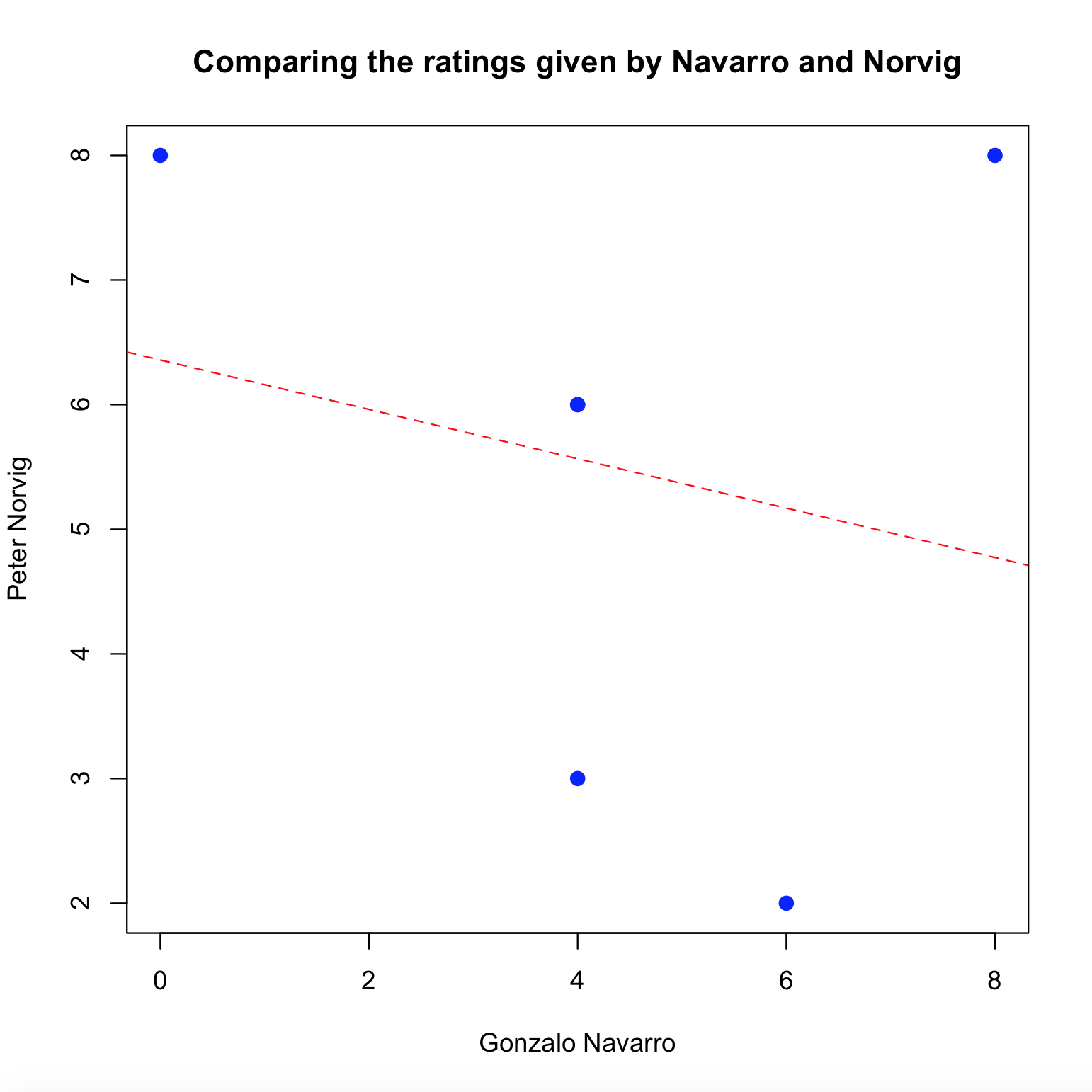
The last plot, shows a negative correlation between Navarro and Norvig.

If we have one dataset $\{x_1, x_2, ..., x_n\}$ containing $n$ elements, and another dataset $\{y_1, y_2, ..., y_n\}$ containing $n$ elements, the formula for the sample PCC is:

$r = \frac{\sum_{i = 1}^{n}(x_i - \bar{x})(y_i - \bar{y})}{\sqrt{\sum_{i = 1}^{n}(x_i-\bar{x})^2} \times \sqrt{\sum_{i = 1}^{n}(y_i-\bar{y})^2}}$

A little algebraic manipulation, yield us to the following formula:

$r = \frac{n\sum{x_iy_i} - \sum x_i\sum y_i}{\sqrt{\left(n\sum x_i^2 - \left( \sum x_i \right) ^ 2\right) \left(n\sum y_i^2 - \left( \sum y_i \right) ^ 2\right)}}$

This formula, let us write a program to compute the PCC between two people.

import math

def pearson_similarity(person1, person2):

    common_ranked_items = [itm for itm in data[person1] \
        if itm in data[person2]]

    n = len(common_ranked_items)

    s1 = sum([data[person1][item] \
        for item in common_ranked_items])
    s2 = sum([data[person2][item] \
        for item in common_ranked_items])

    ss1 = sum([pow(data[person1][item], 2) \
        for item in common_ranked_items])
    ss2 = sum([pow(data[person2][item], 2) \
        for item in common_ranked_items])

    ps = sum([data[person1][item] * data[person2][item] \
        for item in common_ranked_items])

    num = n * ps - (s1 * s2)

    den = math.sqrt((n * ss1 - math.pow(s1, 2)) \
        * (n * ss2 - math.pow(s2, 2)))

    return (num / den) if den != 0 else 0

Both similarity measures allow us to figure it out how similar two people are. The logic behind a recommender system, is to measure everyone against a given person and find the closest people to that specific person, we can do that by taking a group of the people for whom the distance is small, or the similarity is high.

By using this approach, we’re trying to predict what’s going to be the rating if our person rates a group of products he has not rate yet. One of the most used approach to this problem, is to take the ratings of all the other users and multiply how similar they are to the specific person by the rating that they gave to the product. If the product is very popular, and it has been rated by many people, it would have a greater weight, to normalise this behaviour, we do need to divide that weight by the sum of all the similarities for the people that have rated the product. The following function implements this approach.

def recommend(person, bound, similarity):
    # Getting the closest people to person, the number of 
    # elements included in scores, is given by the arg bound
    scores = [(similarity(person, other), other) \
        for other in data if other != person]

    scores.sort()
    scores.reverse()
    scores = scores[0:bound]

    recomms = {}

    for sim, other in scores:
        ranked = data[other]
	    
        for itm in ranked:
            if itm not in data[person]:
                weight = sim * ranked[itm]

                if itm in recomms:
                    s, weights = recomms[itm]
                    recomms[itm] = \
                        (s + sim, weights + [weight])
                else:
                    recomms[itm] = (sim, [weight])

    for r in recomms:
        sim, item = recomms[r]
        recomms[r] = sum(item) / sim

    return recomms

Given a person included in the index (data), a bound (that is maximum number of items to recomend), and a function to measure the similarity between people (euclidean_similarity, or pearson_similarity), this function gives an estimate on how the person would rate the item according to how its similar people rate the item. As an example:

>>> recommend("Alan Perlis", 5, euclidean_similarity)

{
    'Formal methods': 4.2884705749419645,
    'Algorithms': 4.70479765409595, 
    'Computation': 4.39,
    'Concurrency': 4.461820809248555, 
    'Programming language theory': 4.347195972640145
}

>>> recommend("Marvin Minsky", 5, pearson_similarity)

{
    'Formal methods': 4.580731197362096, 
    'Concurrency': 4.242230900860542, 
    'Software engineering': 3.899999999999996, 
    'Programming language theory': 3.4798793670332437
}

>>> recommend("Marvin Minsky", 5, euclidean_similarity)

{
    'Programming language theory': 4.286011590485815, 
    'Databases': 2.8, 
    'Software engineering': 4.272502290210142, 
    'Concurrency': 4.374054188023107, 
    'Formal methods': 3.7690266719570977
}

While Algorithms and Concurrency are perfect topics to recommend to Alan Perlis, or at least that was what our algorithm found, we should keep Marvin Minsky far from the Databases item. There are an strange phenomenon here, depending on the similarity measure, Marvin Minsky seems to like a lot or dislike a little bit the Programming language theory and Formal methods items. By looking for the scores variable while inspecting the code if you call recommend("Marvin Minsky", 5), you can tell that Robin Milner and John McCarthy are the closest to Marvin Minsky, while both Robin Milner and John McCarthy are very different from each other; and also Robin Milner tends to rate a little bit harsher than John McCarthy. That insight clearly taught us that we do need to compare both measures depending on the nature of our data, the election of bound also affects this kind of strange recommendations.

Data exploration, and wrangling comes as significant factors while implementing a production recommender system. The more data it can process, the better recommendations we can give our users. While recommender systems theory is much broader, recommender systems is a perfecto canvas to explore machine learning ideas, algorithms, etc. not only by the nature of the data, but because of the ease visualising and comparing the results.

Resources on Recommender Systems

Programming Collective Intelligence, written by Toby Segaran. Its first chapter includes a math lightweight approach to this amazing topic. It includes an explanation on the two similarity measures explained here, and an approach to match items instead of users, it also includes “big” datasets to play with. The whole book explores machine learning related ideas using a programming-first approach.

Recommender Systems: An Introduction, an academic reference whose first chapter explain with more detail and riguor the material discussed here. Besides math it includes design hints and practical usage of recommender systems. It’s the standard textbook on the topic.

Recommender Systems Specialization, a whole Coursera Specialization on the topic.
The following links provide useful information on deployment of real recommender systems.
- How Recommendation System Works, a review of companies using recommender systems.
- Amazon.com Recommendations, Item-to-Item Collaborative Filtering, a popular-science description of Amazon recommender system written by the engineer that was behind it.
- How does the Amazon Recommendation feature work?, some hints on recommender system design and production-ready artefacts (reading the links related here requires a lot of mathematical maturity and a greedy research enthusiasm).
- How Amazon’s Recommendation System works and What it might be missing
- Now Anyone Can Tap the AI Behind Amazon’s Recommendations
- How does the Netflix movie recommendation algorithm work?

Written on December 19, 2016